datatensor([[ 0.611, -20.199],
[ 4.455, -24.188],
[ 2.071, -20.446],
...,
[ 25.927, 6.597],
[ 18.549, 3.411],
[ 24.617, 8.485]])This post includes a cool animation.
This notebook follows the fastai style guide.
This notebook is based on the contents taught in Lesson 12 of part 2 of the fastai Course, by Jeremy Howard who created the first LLM, ULMFiT in 2016.
Meanshift clustering is a technique for unsupervised learning. Give this algorithm a bunch of data and it will figure out what groups the data can be sorted into. It does this by iteratively moving all data points until they converge to a single point.
The steps of the algorithm can be summarized as follows:
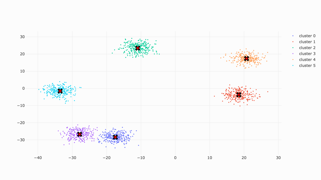
This is the data we will work with to illustrate meanshift clustering. The data points are put into clearly seperate clusters for the sake of clarity.
In the end, all clusters will converge at their respective center (marked by X).
Let’s start off simple and apply the algorithm to a single point.
For each data point \(x\) in the dataset, calculate the distance between \(x\) and every other data point in the dataset.
datatensor([[ 0.611, -20.199],
[ 4.455, -24.188],
[ 2.071, -20.446],
...,
[ 25.927, 6.597],
[ 18.549, 3.411],
[ 24.617, 8.485]])X = data.clone(); X.shapetorch.Size([1500, 2])Each point has an \(x\) coordinate and a \(y\) coordinate.
x = X[0, :]; x - Xtensor([[ 0.000, 0.000],
[ -3.844, 3.989],
[ -1.460, 0.247],
...,
[-25.316, -26.796],
[-17.938, -23.610],
[-24.006, -28.684]])The distance metric we’ll use is Euclidean distance — also better known as Pythagoras’ theorem.
\[ \sqrt{(x_2 - x_1)^2 + (y_2 - y_1)^2} \]
dists = (x - X).square().sum(dim=1).sqrt(); diststensor([ 0.000, 5.540, 1.481, ..., 36.864, 29.651, 37.404])Calculate weights for each point in the dataset by passing the calculated distances through the normal distribution.
The normal distribution is also known as the Gaussian distribution. A distribution is simply a way to describe how data is spread out — this isn’t applicable in our case. What is applicable is the shape of this distribution which we will use to calculate the weights.
\[ f(x) = \frac{1}{\sigma \sqrt{2\pi} } e^{-\frac{1}{2}\left(\frac{x-\mu}{\sigma}\right)^2} \]
def gauss_kernel(x, mean, std):
  return torch.exp(-(x - mean) ** 2 / (2 * std ** 2)) / (std * torch.sqrt(2 * tensor(torch.pi)))
This is how it looks like.
From the shape of this graph, we can see that larger values of \(x\) give smaller values of \(y\), which is what we want — longer distances should have smaller weights meaning they have a smaller effect on the new position of the point.
We can control the rate at which the weights go to zero by varying what’s known as the bandwidth, or the standard deviation. The graph above is generated with a bandwith of 2.5.
The graph below is generated with a bandwidth of 1.
Let’s get our weights now.
gauss_kernel(dists, mean=0, std=2.5)tensor([ 0.160, 0.014, 0.134, ..., 0.000, 0.000, 0.000])bw = 2.5
ws = gauss_kernel(x=dists, mean=0, std=bw)Calculate the weighted average for all points in the dataset. This weighted average is the new location for \(x\)
ws.shape, X.shape(torch.Size([1500]), torch.Size([1500, 2]))ws[:, None].shape, X.shape(torch.Size([1500, 1]), torch.Size([1500, 2]))Below is the formula for weighted average.
\[ \frac{\sum wx}{\sum w} \]
In words, multiply each data point in the set with its corresponding weight and sum all products. Divide that with the sum of all weights.
ws[:, None] * X, ws[0] * X[0, :](tensor([[ 0.097, -3.223],
[ 0.061, -0.331],
[ 0.277, -2.738],
...,
[ 0.000, 0.000],
[ 0.000, 0.000],
[ 0.000, 0.000]]),
tensor([ 0.097, -3.223]))Let’s calculate the weighted average and assign it as the new location for our point \(x\).
x = (ws[:, None] * X).sum(dim=0) / ws.sum(); xtensor([ 1.695, -20.786])And there you have it! We just moved a single data point.
Let’s do this for all data points and for a single iteration.
for i, x in enumerate(X):
    dist = (x - X).square().sum(dim=1).sqrt()
    ws = gauss_kernel(x=dist, mean=0, std=bw)
X[i] = (ws[:, None] * X).sum(dim=0) / ws.sum()plot_data(centroids+2, X, n_samples)Let’s encapsulate the algorithm so we can run it for multiple iterations.
def update(X):
    for i, x in enumerate(X):
      dist = (x - X).square().sum(dim=1).sqrt()
      ws = gauss_kernel(x=dist, mean=0, std=bw)
      X[i] = (ws[:, None] * X).sum(dim=0) / ws.sum()

def meanshift(data):
   X = data.clone()
   for _ in range(5): update(X)
return Xplot_data(centroids+2, meanshift(data), n_samples)All points have converged.
%timeit -n 10 meanshift(data)1.7 s ± 282 ms per loop (mean ± std. dev. of 7 runs, 10 loops each)The algorithm took roughly 1.5 seconds to run 5 iterations. We’ll optimize the algorithm further in Optimized Implementation.
As we can see below, simply moving the algorithm to the GPU won’t help — in fact, it becamse a bit slower.
def update(X):
    for i, x in enumerate(X):
      dist = (x - X).square().sum(dim=1).sqrt()
      ws = gauss_kernel(x=dist, mean=0, std=bw)
      X[i] = (ws[:, None] * X).sum(dim=0) / ws.sum()

def meanshift(data):
   X = data.clone().to('cuda')
   for _ in range(5): update(X)
   return X.detach().cpu()

%timeit -n 10 meanshift(data)
1.67 s ± 49.7 ms per loop (mean ± std. dev. of 7 runs, 10 loops each)Let’s see meanshift clustering happen in real time.
X = data.clone()
fig = plot_data(centroids+2, X, n_samples, display=False)
fig.update_layout(xaxis_range=[-40, 40], yaxis_range=[-40, 40],  updatemenus=[dict(type='buttons', buttons=[
    dict(label='Play', method='animate', args=[None]),
    dict(label='Pause', method='animate', args=[[None], dict(frame_duration=0, frame_redraw='False', mode='immediate', transition_duration=0)])
])])

frames = [go.Frame(data=fig.data)]
for _ in range(5):
    update(X)
    frames.append(go.Frame(data=plot_data(centroids+2, X, n_samples, display=False).data))
fig.frames = frames
fig.show()The implementation above is roughly 1.5s which is slow. Let’s perform the algorithm on multiple data points simulataneously. We’ll then move the operations onto the GPU.
For each data point \(x\) in the dataset, calculate the distance between \(x\) and every other data point in the dataset.
X = data.clone(); X.shapetorch.Size([1500, 2])We’ll begin with a batch size of 8.
bs = 8
x = X[:bs, :]; x
tensor([[ 0.611, -20.199],
[ 4.455, -24.188],
[ 2.071, -20.446],
[ 1.011, -23.082],
[ 4.516, -22.281],
[ -0.149, -22.113],
[ 4.029, -18.819],
[ 2.960, -18.646]])x.shape, X.shape(torch.Size([8, 2]), torch.Size([1500, 2]))x[:, None, :].shape, X[None, ...].shape(torch.Size([8, 1, 2]), torch.Size([1, 1500, 2]))x[:, None, :] - X[None, ...]tensor([[[ 0.000, 0.000],
[ -3.844, 3.989],
[ -1.460, 0.247],
...,
[-25.316, -26.796],
[-17.938, -23.610],
[-24.006, -28.684]],
[[ 3.844, -3.989],
[ 0.000, 0.000],
[ 2.383, -3.742],
...,
[-21.472, -30.786],
[-14.094, -27.599],
[-20.162, -32.673]],
[[ 1.460, -0.247],
[ -2.383, 3.742],
[ 0.000, 0.000],
...,
[-23.856, -27.043],
[-16.477, -23.857],
[-22.546, -28.931]],
...,
[[ -0.759, -1.914],
[ -4.603, 2.076],
[ -2.220, -1.667],
...,
[-26.076, -28.710],
[-18.697, -25.523],
[-24.766, -30.598]],
[[ 3.418, 1.380],
[ -0.426, 5.369],
[ 1.958, 1.627],
...,
[-21.898, -25.417],
[-14.520, -22.230],
[-20.588, -27.304]],
[[ 2.349, 1.553],
[ -1.495, 5.542],
[ 0.889, 1.800],
...,
[-22.967, -25.243],
[-15.589, -22.057],
[-21.657, -27.131]]])(x[:, None, :] - X[None, ...]).shapetorch.Size([8, 1500, 2])dists = (x[:, None, :] - X[None, ...]).square().sum(dim=-1).sqrt(); dists, dists.shape(tensor([[ 0.000, 5.540, 1.481, ..., 36.864, 29.651, 37.404],
[ 5.540, 0.000, 4.437, ..., 37.534, 30.989, 38.394],
[ 1.481, 4.437, 0.000, ..., 36.062, 28.994, 36.679],
...,
[ 2.059, 5.050, 2.776, ..., 38.784, 31.639, 39.364],
[ 3.686, 5.386, 2.546, ..., 33.549, 26.552, 34.196],
[ 2.816, 5.740, 2.007, ..., 34.128, 27.009, 34.715]]),
torch.Size([8, 1500]))Calculate weights for each point in the dataset by passing the calculated distances through the normal distribution.
We can simplify the guassian kernel to a triangular kernel and still achieve the same results, with less computation.
plot_func(partial(gauss_kernel, mean=0, std=2.5))def tri_kernel(x, bw): return (-x+bw).clamp_min(0)/bw
plot_func(partial(tri_kernel, bw=8))%timeit gauss_kernel(dists, mean=0, std=2.5)311 µs ± 8.06 µs per loop (mean ± std. dev. of 7 runs, 1000 loops each)%timeit tri_kernel(dists, bw=8)25 µs ± 594 ns per loop (mean ± std. dev. of 7 runs, 10000 loops each)gauss_kernel(dists, mean=0, std=2.5), tri_kernel(dists, bw=8)(tensor([[ 0.160, 0.014, 0.134, ..., 0.000, 0.000, 0.000],
[ 0.014, 0.160, 0.033, ..., 0.000, 0.000, 0.000],
[ 0.134, 0.033, 0.160, ..., 0.000, 0.000, 0.000],
...,
[ 0.114, 0.021, 0.086, ..., 0.000, 0.000, 0.000],
[ 0.054, 0.016, 0.095, ..., 0.000, 0.000, 0.000],
[ 0.085, 0.011, 0.116, ..., 0.000, 0.000, 0.000]]),
tensor([[1.000, 0.308, 0.815, ..., 0.000, 0.000, 0.000],
[0.308, 1.000, 0.445, ..., 0.000, 0.000, 0.000],
[0.815, 0.445, 1.000, ..., 0.000, 0.000, 0.000],
...,
[0.743, 0.369, 0.653, ..., 0.000, 0.000, 0.000],
[0.539, 0.327, 0.682, ..., 0.000, 0.000, 0.000],
[0.648, 0.282, 0.749, ..., 0.000, 0.000, 0.000]]))ws = tri_kernel(dists, bw=8); ws.shapetorch.Size([8, 1500])Calculate the weighted average for all points in the dataset. This weighted average is the new location for \(x\)
ws.shape, X.shape(torch.Size([8, 1500]), torch.Size([1500, 2]))ws[..., None].shape, X[None, ...].shape(torch.Size([8, 1500, 1]), torch.Size([1, 1500, 2]))(ws[..., None] * X[None, ...]).shapetorch.Size([8, 1500, 2])(ws[..., None] * X[None, ...]).sum(1).shapetorch.Size([8, 2])%timeit (ws[..., None] * X[None, ...]).sum(1)144 µs ± 31.2 µs per loop (mean ± std. dev. of 7 runs, 10000 loops each)Let’s have another look at formula for weighted average.
\[ \frac{\sum wx}{\sum w} \]
The numerator is actually the definition for matrix multiplication! Therefore we can speed up the operation above by using the @ operator!
%timeit ws @ X7.64 µs ± 184 ns per loop (mean ± std. dev. of 7 runs, 100000 loops each)A roughly 40% speed up!
x = (ws @ X) / ws.sum(dim=1, keepdim=True); xtensor([[ 2.049, -20.954],
[ 3.108, -21.923],
[ 2.441, -21.021],
[ 2.176, -21.616],
[ 3.082, -21.466],
[ 1.842, -21.393],
[ 2.946, -20.632],
[ 2.669, -20.594]])And there you have it! We performed this algorithm on 8 data points simultaneously!
Let’s encapsulate the code so we can perform it over all data points and time it.
?slicebs8min(1508, 1500)1500X = data.clone()
n = len(data)
bs = 8
for i in range(0, n, bs):
s = slice(i, min(i+bs, n))
dists = (X[s][:, None, :] - X[None, ...]).square().sum(dim=-1).sqrt()
ws = egauss_kernel(dists, mean=0, std=2.5)
X[s] = (ws @ X) / ws.sum(dim=1, keepdim=True)plot_data(centroids+2, X, n_samples)def update(X):
for i in range(0, n, bs):
s = slice(i, min(i+bs, n))
dists = (X[s][:, None, :] - X[None, ...]).square().sum(dim=-1).sqrt()
ws = egauss_kernel(dists, mean=0, std=2.5)
X[s] = (ws @ X) / ws.sum(dim=1, keepdim=True)
def meanshift(data):
X = data.clone()
for _ in range(5): update(X)
return Xplot_data(centroids+2, meanshift(data), n_samples)%timeit -n 10 meanshift(data)700 ms ± 43.4 ms per loop (mean ± std. dev. of 7 runs, 10 loops each)From 1.5 seconds to 0.5 seconds! A 3x speed increase — very nice!
Let’s move onto the GPU and now see what improvements we get.
def meanshift(data):
   X = data.clone().to('cuda')
   for _ in range(5): update(X)
   return X.detach().cpu()

%timeit -n 10 meanshift(data)
263 ms ± 27.4 ms per loop (mean ± std. dev. of 7 runs, 10 loops each)0.5s to 0.25s — a 2x speed increase!
Meanshift clustering simply involves moving points, by taking into account surrounding points, iteratively until they converge.
If you have any comments, questions, suggestions, feedback, criticisms, or corrections, please do post them down in the comment section below!