Stable Diffusion, Summarized

Taking a Look at how Diffusers Dream

A concise, high level overview on the mechanisms of stable diffusion.

This post was edited on Sunday, 30 April 2023

Here, I explain the workings of stable diffusion at a high level.

Components

A diffuser contains four main components

• The text encoder
• The image encoder
• The autoencoder (VAE autoencoder)
• The neural network (U-net)

flowchart TB
    A{{Diffuser}}
    B([U-net])
    C([VAE Autoencoder])
    D([Text Encoder])
    E([Image Encoder])

    A --> D & E & C & B

Training

I’ll explain the training process in terms of a single image.

When all components shown above are put into their respective places, the overall training process looks like this.

flowchart LR
    subgraph A [Feature Vector Creation]
        id1([Text Encoder])
        id2([Image Encoder])
    end

    subgraph B [Image Compression]
        id3([VAE Autoencoder])
    end

    subgraph C [Noise Removal]
        id4([U-net])
    end

    subgraph D [Image Decompression]
        id5([VAE Autoencoder])
    end

    id7[Input Image Description] & id6[Input Image] --> A --> id9[Feature Vector]
    id6 --> B --noise added to image--> id10[Noisy Latent]
    id9 & id10 --> C --> id11[Less Noisy Latent] -->  C
    id11 --> D --> id8[Generated Image]

Let’s break it down.

Feature Vector Creation

flowchart TB
    subgraph B [ ]
        direction LR
        id1[Input Image]
        id2[Input Image Description]
        subgraph A [Feature Vector Creation]
            id3([Text Encoder])
            id4([Image Encoder])
        end
        id2 & id1 --> A --> id11[Feature Vector]
    end
    style B fill:#FFF, stroke:#333,stroke-width:3px

    subgraph C [ ]
        direction LR
        id5[Input Image]
        id7[Input Image Descripton]
        id5 --> id6
        id7 --> id8
        subgraph D [Feature Vector Creation]
            id6([Image Encoder])
            id8([Text Encoder])
            id6 & id8 --> id9[CLIP Embedding]
        end
        id9 --> id10[Feature Vector]
    end
    style C fill:#FFF, stroke:#333,stroke-width:3px

    B --> C
    B --> C
    B --> C

We start with an image and its description. The image encoder takes the image and produces a feature vector — a vector with numerical values that describe the image in some way. The text encoder takes the image’s description and similarly produces a feature vector.

These two feature vectors are then stored in what’s known as a CLIP embedding. An embedding is simply a table where each row is an item and each column describes the items in some way. In this case, the rows represent feature vectors, and the columns are each feature in the vector.

Both encoders keep producing feature vectors until they are as similar as possible.

Image Compression

flowchart TB
    subgraph A [ ]
        id2[Input Image] --> id1
        subgraph B [Image Compression]
            direction LR
            id1([VAE Autoencoder])
        end
        id1 --> id7[Latent]
    end
    style A fill:#FFF, stroke:#333,stroke-width:3px

    subgraph C[ ]
        direction LR
        id3[Input Image]
        subgraph D [Image Compression]
            id4([VAE Encoder])
            id5([VAE Decoder])
        end
        id3 --> id4 --> id6[Latent]
    end
    style C fill:#FFF, stroke:#333,stroke-width:3px

    A & A & A --> C

Once the feature vectors have been produced, the image is compressed by the VAE autoencoder. Some noise is then tossed onto the image.

The VAE autoencoder contains an encoder and a decoder. The encoder handles compression whereas the decoder handles decompression.

The compressed noisy image is now known as the latent. The image is compressed for faster computation, as there would be fewer pixels to compute on.

Noise Removal

flowchart TB
    subgraph A [ ]
        id1[Feature Vector] & id2[Noisy Latent] --> id3
        subgraph B [Noise Removal]
            direction LR
            id3([U-net]) --> id4[Noise]
        end
        id4 --with learning rate--> id5[Less Noisy Latent] --> id3
    end
    style A fill:#FFF, stroke:#333,stroke-width:3px 

    subgraph C [ ]
        id6[Feature Vector] & id7[Noisy Latent] --> id8
        subgraph Noise Removal
            direction LR
            id8([U-net])
        end
        id8 --> id9([Less Noisy Latent]) --> id8
    end
    C & C & C --> A
    style C fill:#FFF, stroke:#333,stroke-width:3px

The latent, together with its feature vector, is now input to the U-net. Instead of predicting what the original, un-noisy image was, the U-net predicts the noise that was tossed onto the image.

Once it outputs the predicted noise, that noise is subtracted from the latent in conjunction with the learning rate. This new, less noisy latent is now input again and the process repeats until desired.

Image Decompression

flowchart TB
    subgraph A [ ]
        direction LR
        id2[Input Image] --> id1
        subgraph B [Image Decompression]
            id1([VAE Autoencoder])
        end
        id1 --> id7[Latent]
    end
    style A fill:#FFF, stroke:#333,stroke-width:3px

    subgraph C [ ]
        direction LR
        id3[Less Noisy Latent] --> id5
        subgraph D [Image Decompression]
            id4([VAE Encoder])
            id5([VAE Decoder])
        end
        id5 --> id6[Generated Image]
    end
    style C fill:#FFF, stroke:#333,stroke-width:3px

    A & A & A --> C

The latent is now decompressed through the VAE autoencoder’s decoder.

We now have a generated image!

Inference

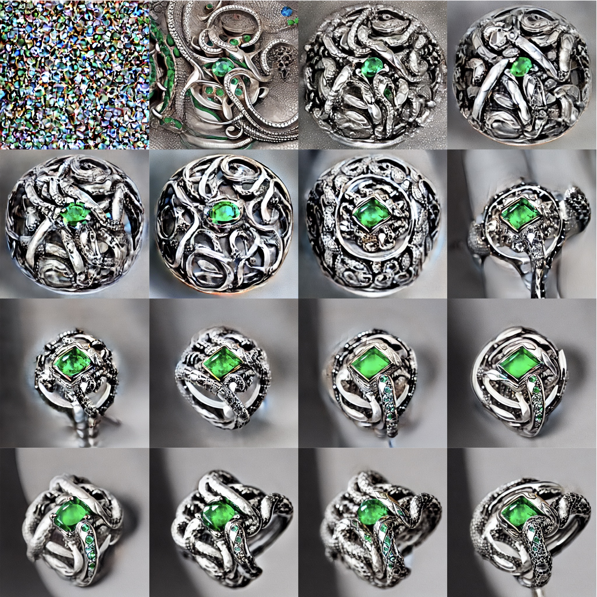
When using a diffuser for inference, the diffuser typically begins with a purely noisey latent. The diffuser uses the input prompt to guide the removal of noise from the latent, until the latent resembles what is desired.

Conclusion

And that’s all there is to it!

We take an image and its prompt, and create a feature vector out of them. The image is compressed and noise is then added to it. The latent and the feature vector are input to a U-net which then predicts the noise in the latent. The predicted noise is subtracted from the latent, which is then input back to the U-net. After the desired number of steps has lapsed, the latent is decompressed and the generated image is ready!

If you have any comments, questions, suggestions, feedback, criticisms, or corrections, please do post them down in the comment section below!